Introduction

Fix a number \(\alpha > 0\). We look at the mapping that takes a discrete distribution \(P\) and outputs a new distribution \(Q\) defined by \[Q(a) ~=~ \frac{P(a)^\alpha}{\sum_a P(a)^\alpha} .\] This mapping is sometimes called the escort probability map (I do not know yet why). It is a continuous bijection from the simplex to itself. It maps the uniform distribution to itself, and corners to corners. For \(\alpha=1\) it is the identity mapping.

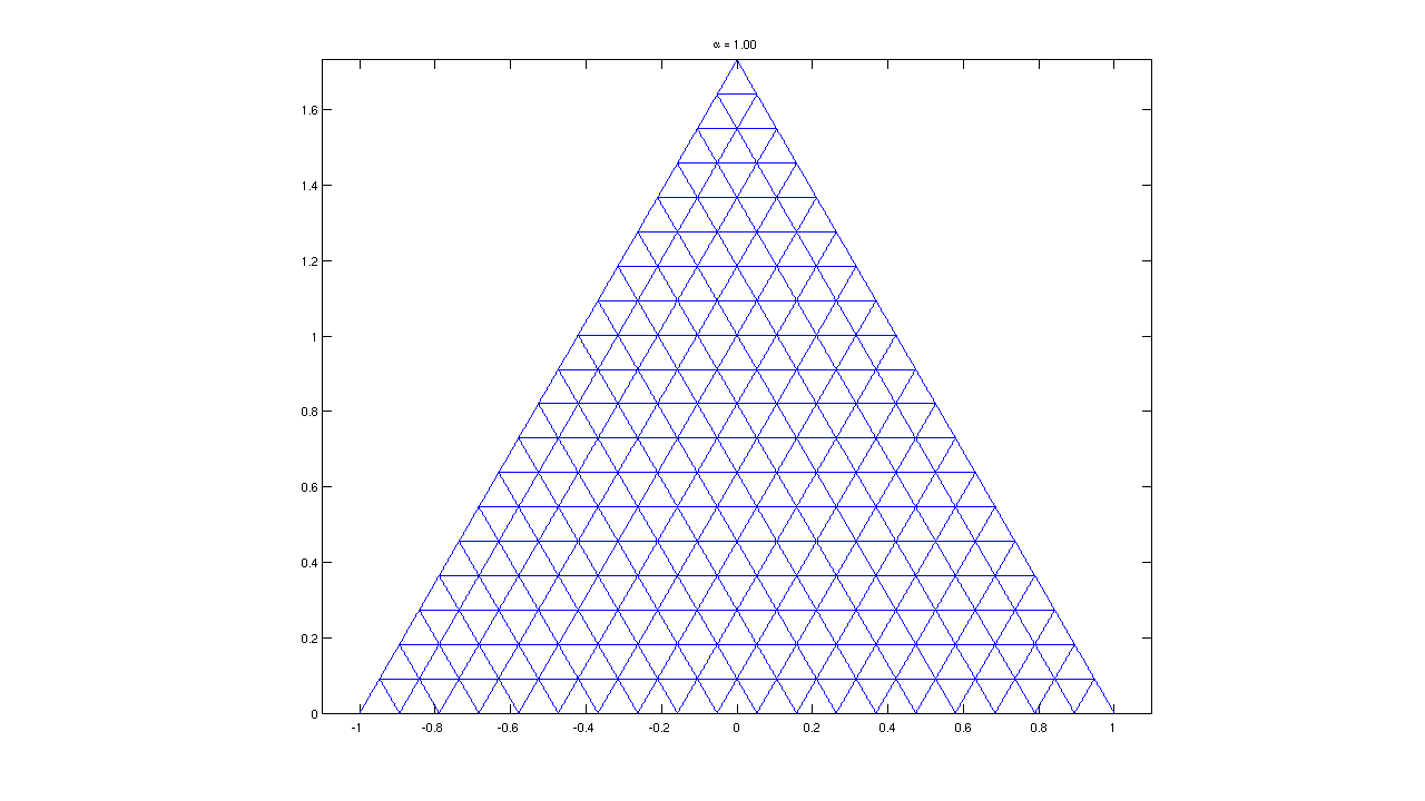
To get a feeling for the effect of \(\alpha\), let us put a regular triangular mesh on the 3 simplex. We can then graph the mesh after applying the escort probability map. For \(\alpha=1\) we recover the input mesh:

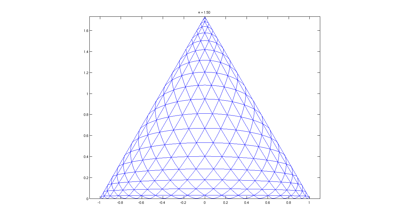
Now let’s see what happens for \(\alpha > 1\). We see that distributions are pushed towards the corners.

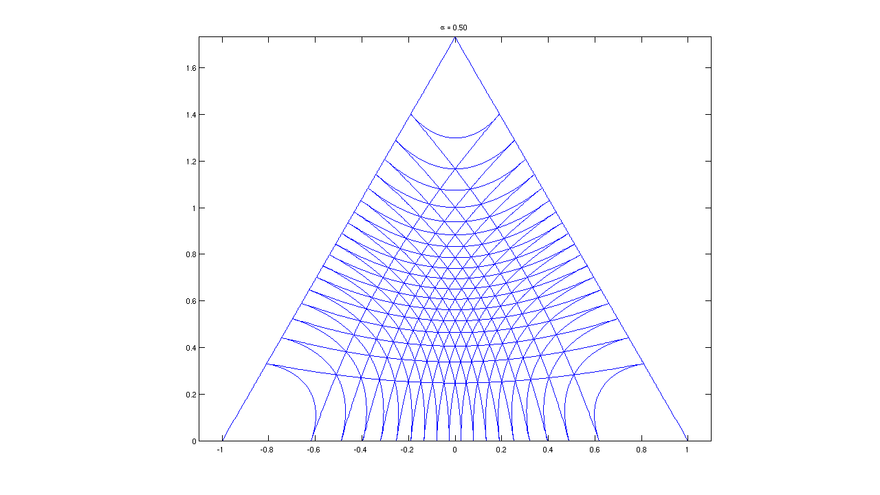
and similarly for \(\alpha < 1\) distributions are sucked toward the middle

Here is a video interpolating smoothly from \(\alpha=0\) to \(\alpha=2\).