2017-03-11
A Droste image contains a smaller copy of itself. We look at how to render such images.
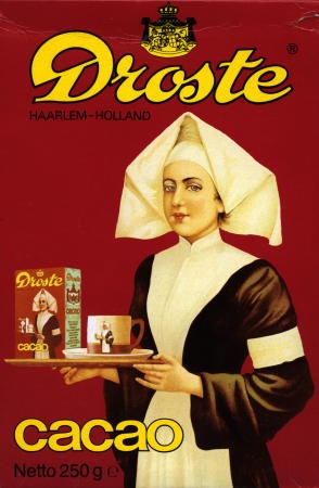
This post is about images that contain themselves. A famous such image appears on the Droste cacao box (whence the name Droste effect):
In this post we will look at rendering images with one or more Droste effects.
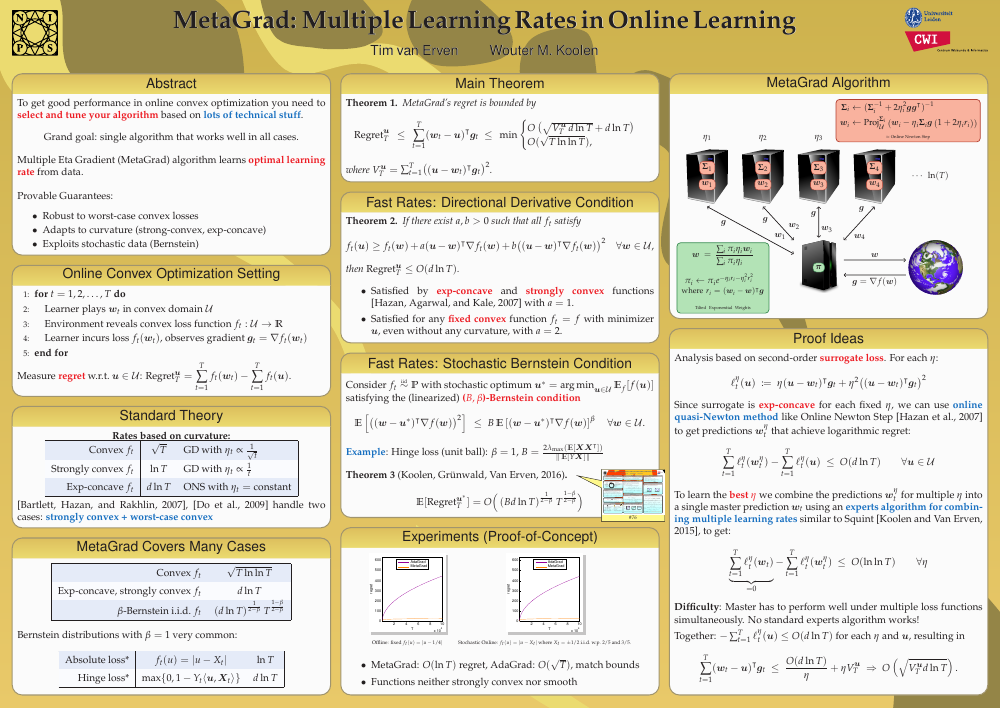
Here is my reason for getting interested in the Droste effect. This December I presented two papers at the NIPS’16 conference in Barcelona. Accepted papers at NIPS are presented in a poster session. So I made two posters. Now these papers are on two aspects of the same topic, and so they naturally refer to each other (i.e. each cites the other). To represent this visually in the posters, I had each poster include a little picture of the other poster:
 |
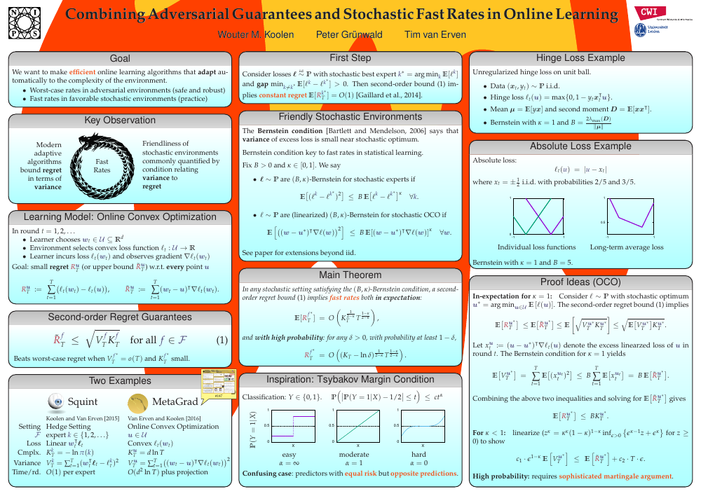 |
If you think about it, each poster therefore contains a smaller copy of itself (by following the inclusion two levels deep). This immediately leads to a compilation conundrum. To compile the one poster we need the PDF of the other, and vice versa. I ended up solving this iteratively, by starting with empty posters PDFs, and then compiling the posters back and forth three times. As the posters shrink a lot with each inclusion, three times was enough to create PDFs that were visually indistinguishable from perfect infinite regress. However, this process does result in a large file size, as all the included copies of each poster are stored separately in the PDFs.
To me, replicating nested copies seems wasteful. This leads to the main question of this post: Can we build an efficient graphics system that includes a Droste operator primitive? The Droste operator would mean: include the full picture translated and shrunk by such and such amounts. The task of the system would then be to render the specified image to a bitmap (i.e. for displaying or printing).
So here is what I came up with.
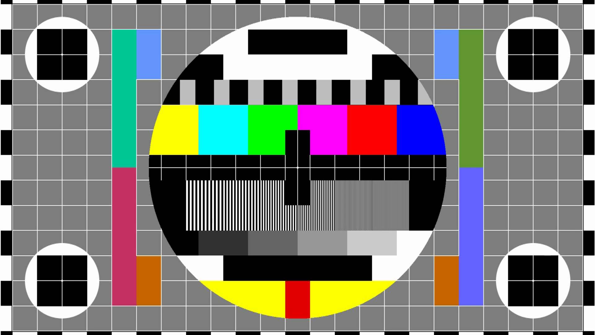
Let me start by showing the result. I will use this test image as the background to have something to Drostify:
Now let’s put a Droste effect on this image. Or, to make things more interesting, let’s put three. I will be working off this small specification:
| 1. Include image “test” |
| 2. Add Droste centered at (.325, .40) shrunk by .6 |
| 3. Add Droste centered at (.800, .20) shrunk by .1 |
| 4. Add Droste centered at (.825, .75) shrunk by .3 |
This specification is an instruction to apply 3 Droste operations in the following areas:

And here is the resulting image rendered (using the code at the end of this post which implements the method sketched below):
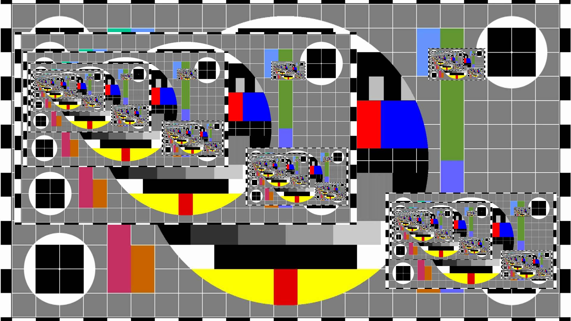
An easy way to render the above specification is as follows. As our first (bad) approximation, we take the test image itself. We then iteratively refine. In iteration \(i+1\), we render the test image, and we render at each Droste spot an appropriately scaled copy of the \(i\)th image. We keep on doing so until convergence.
Although simple, this method has a couple of disadvantages
It is inefficient: we are rendering stable parts of the image many times.
Errors (due to the rounding in the rescaling) accumulate.
In practice it does not quite converge. It oscillates between a few indistinguishable versions of the image.
This raises the question whether we can render the entire image in a single shot.
The idea to render a Droste specification like the above is as follows. For each point \((x,y)\) in the to-be-rendered output image, we compute the location in the input test image whose colour we should display there. For the points outside all Droste regions this is easy: these points map to themselves. The color value of a point inside a Droste region comes from some other point outside. Which point? Let’s figure out how that works.
It is easiest to think of a spherical image and a spherical Droste region, as a sphere only has one boundary whereas a rectangle has four. So let the entire picture be a unit circle. Consider first a single Droste operator at position \(\boldsymbol{p}\) with radius \(\rho < 1\). Here is a diagram of how that looks and what happens:

As you can see, Droste operation has a vanishing point (and, interestingly, the colour at this vanishing point can be chosen arbitrarily). The vanishing point is located at \[\boldsymbol{s} ~=~ \sum_{s=0}^\infty \rho^s \boldsymbol{p} ~=~ \frac{\boldsymbol{p}}{1-\rho} .\] The points that are in the first copy (red circle) are those points \(\boldsymbol{x}\) for which \(\left\|\boldsymbol{p}-\boldsymbol{x}\right\| \le \rho\). The points in the second copy (green circle) are those for which \(\left\|\boldsymbol{x}- \boldsymbol{p}(1+\rho)\right\| \le \rho^2\). Those in the \(i\)th copy are those for which \[\rho^i ~\ge~ \left\|\boldsymbol{x}- \boldsymbol{p}\sum_{s=0}^{i-1} \rho^s\right\| ~=~ \left\|\boldsymbol{x}- \boldsymbol{p}\frac{1-\rho^i}{1-\rho}\right\| ~=~ \left\|\boldsymbol{x}- \boldsymbol{s}+ \boldsymbol{s}\rho^i\right\| ~=~ \sqrt{ \left\|\boldsymbol{x}- \boldsymbol{s}\right\|^2 + 2 (\boldsymbol{x}- \boldsymbol{s})^\intercal\boldsymbol{s}\rho^i + \left\|\boldsymbol{s}\rho^i\right\|^2 }\] which we may square to \[\rho^{2 i} ~\ge~ \left\|\boldsymbol{x}- \boldsymbol{s}\right\|^2 + 2 \rho^i (\boldsymbol{x}- \boldsymbol{s})^\intercal\boldsymbol{s} + \rho^{2 i} \left\|\boldsymbol{s}\right\|^2\] So the largest integer \(i\) satisfying the above requirement (i.e. the nesting level of \(\boldsymbol{x}\)) is \[i(\boldsymbol{x}) ~=~ \left\lfloor\ln_\rho \left(\frac{b + \sqrt{b^2+c a}}{a}\right)\right\rfloor\] where \begin{align*} a &~=~ 1 - \|\boldsymbol{s}\|^2, & b &~=~ (\boldsymbol{x}-\boldsymbol{s})^\intercal\boldsymbol{s}, & c &~=~ \|\boldsymbol{x}-\boldsymbol{s}\|^2 . \end{align*} And hence the input point whose colour we should display at \(\boldsymbol{x}\) is \[f_{\boldsymbol{p},\rho}(\boldsymbol{x}) ~=~ \boldsymbol{s}+ (\boldsymbol{x}-\boldsymbol{s}) \rho^{-i(\boldsymbol{x})} .\] To render an image with a single Droste region, we assign to each output pixel \(\boldsymbol{x}\) the colour at input pixel \(\boldsymbol{x}' = f_{(\boldsymbol{p},\rho)}(\boldsymbol{x})\). If the input image is a bitmap and \(\boldsymbol{x}'\) falls between pixels we interpolate the values of its neighbouring pixels appropriately.
Images with multiple Droste regions are more complicated, as we can see each region in all others. Still, we can render it by determining the colour of each output pixel \(\boldsymbol{x}\). The colour comes from some input pixel \(\boldsymbol{x}'\) which we determine iteratively. We start by setting \(\boldsymbol{x}'=\boldsymbol{x}\). We then iterate over the list of Droste operators, and for each Droste operator \((\boldsymbol{p},\rho)\), we apply \(\boldsymbol{x}' \mapsto f_{(\boldsymbol{p},\rho)}(\boldsymbol{x}')\). We keep on doing this until \(\boldsymbol{x}'\) is outside all Droste regions. Then we assign to \(\boldsymbol{x}\) the colour of the input image at \(\boldsymbol{x}'\).
The above method resolves each individual Droste operator in a single shot. But it does not resolve multiple Droste operators. It would be interesting to see if an entire constellation of Droste operators can be resolved analytically. I doubt it, though.
Neighbouring output pixels typically come from neighbouring input pixels (but not so on the boundary of Droste regions). Can we use this to render faster?
Here is the Octave code I used to generate the above Drostified test image.
| goback.m | Octave render script |
| bkup.cpp | MEX file |
| test.jpg | Input image |
Within Octave, first compile the MEX file using mex bkup.cpp and then run the renderer with goback.